Bienvenue au Laboratoire d'Optique Atmosphérique
Unité Mixte de Recherche (CNRS / Lille 1) située sur le campus de l'Université Lille 1 à Villeneuve d'Ascq, dont le rôle est principalement l'observation et la modélisation des propriétés de l'atmosphère.
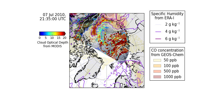
Impact des aérosols sur la microphysique des nuages en Arctique
Corrélation entre microphysique des nuages, panaches de feux et paramètres météorologiques
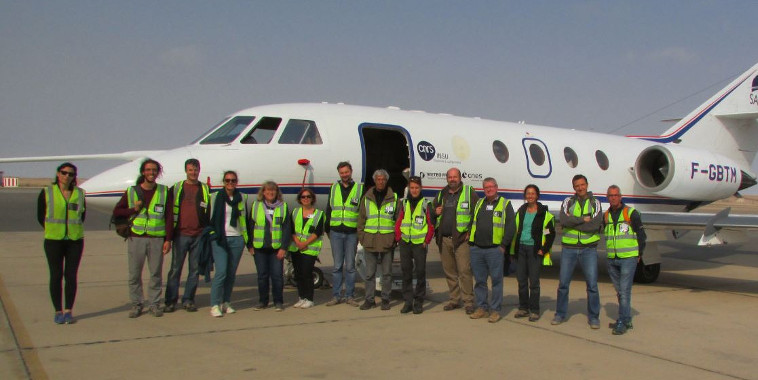
Premiers résultats de la campagne de mesures AEROCLO-SA
qui s'est déroulée en Namibie du 22 août au 12 septembre 2017
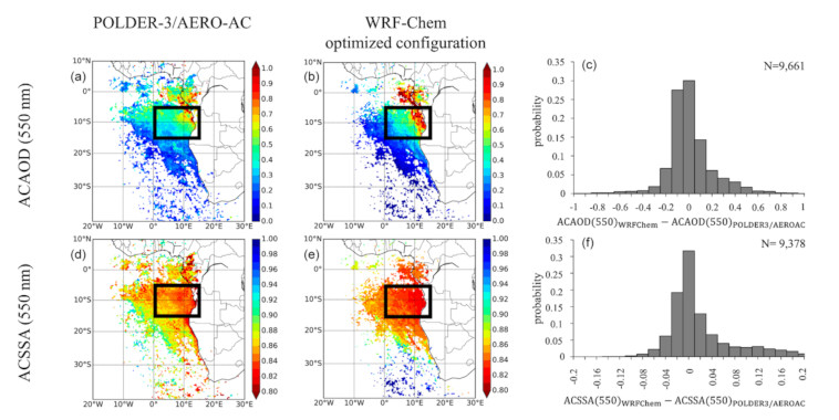
Modélisation et télédétection satellitaire des propriétés optiques des aérosols de feux de biomasse de la région de l’Atlantique sud-est
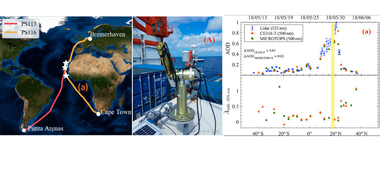
Premières mesures d'aérosols avec un photomètre Sun-Sky-Lunaire sur bateau
Lidar de polarisation Raman à plusieurs longueurs d'ondes colocalisé au niveau de l'océan Atlantique
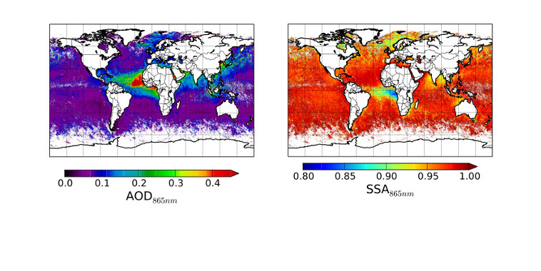
Distribution globale de l'absorption des aérosols (SSA)
pour la première fois inversée dans le proche-infrarouge (POLDER) et concentration associée (AOD)
Changement climatique : même les nuages ne sont plus ce qu'ils étaient !
Plongez dans les mystères des nuages et découvrez comment le changement climatique les transforme ! Cet article de La Voix du Nord nous emmène à la rencontre des chercheurs lillois qui scrutent les cieux pour comprendre l'évolution de ces géants cotonneux.
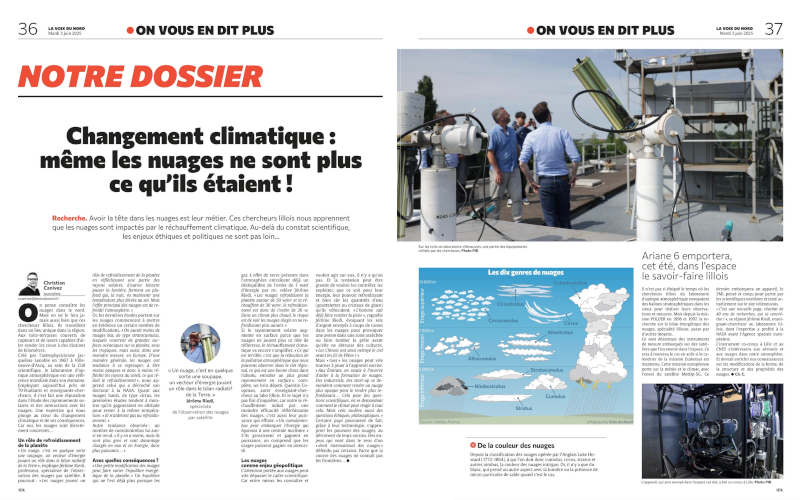
Une aventure scientifique qui révèle que même les nuages ne sont plus ce qu'ils étaient, avec des impacts insoupçonnés sur notre climat.
Retrouvez l'intégralité de cet article sur le site Cafeyn.
MAP-IO: an atmospheric and marine observatory program on board Marion Dufresne over the Southern Ocean
Tulet, P., Van Baelen, J., Bosser, P., Brioude, J., Colomb, A., Goloub, P., Pazmino, A., Portafaix, T., Ramonet, M., Sellegri, K., Thyssen, M., Gest, L., Marquestaut, N., Mékiès, D., Metzger, J.-M., Athier, G., Blarel, L., Delmotte, M., Desprairies, G., Dournaux, M., Dubois, G., Duflot, V., Lamy, K., Gardes, L., Guillemot, J.-F., Gros, V., Kolasinski, J., Lopez, M., Magand, O., Noury, E., Nunes-Pinharanda, M., Payen, G., Pianezze, J., Picard, D., Picard, O., Prunier, S., Rigaud-Louise, F., Sicard, M. & Torres, B.
Derivation of depolarization ratios of aerosol fluorescence and water vapor Raman backscatters from lidar measurements
Veselovskii, I., Hu, Q., Goloub, P., Podvin, T., Boissiere, W., Korenskiy, M., Kasianik, N., Khaykyn, S. & Miri, R.
Growth and Global Persistence of Stratospheric Sulfate Aerosols From the 2022 Hunga Tonga–Hunga Ha'apai Volcanic Eruption
Boichu, M., Grandin, R., Blarel, L., Torres, B., Derimian, Y., Goloub, P., Brogniez, C., Chiapello, I., Dubovik, O., Mathurin, T., Pascal, N., Patou, M. & Riedi, J.
Villeneuve d'Ascq (alt. 60m)

- Température
- 17.3° C
- Pression abs.
- 1026.9 hPa
Mis à jour le 3 juil. 2025, 6h30 TUC